My post on Moon Tracking covers most of the complexities involved in tracking things, but not quite everything. I chose to talk about the Moon first because it covered all of the most complex parts of the tracker. This post covers all of the rest of the things that the Cosmic Signpost can currently track.

Planets

Tracking planets in our solar system is only a small addition to the complexity of tracking the Moon.

JPL provides some approximate orbital parameters for tracking planets. They’re fairly simple models, so won’t be particularly accurate, but they’ve very simple to implement and given the distance from Earth the inaccuracies won’t be very noticeable.

However, they are all based on a heliocentric inertial reference frame. We have our ECI frame though, and the axes are in the same directions, so we should be able to subtract out the Earth’s position vector to get to that frame, right?

Unfortunately, the orbital parameters that JPL gives for Earth are actually the Earth-Moon-Barycentre. The Barycentre of a set of objects is the centre of mass of all of them together, and in the case of the Earth-Moon system, the Barycentre is about 4,671 km from the centre of the Earth, or most of the distance from the centre of the Earth to the crust. Since we already know how to track the Moon, we can track the Earth-Moon-Barycentre by multiplying the Moon’s position vector (from Earth) by the ratio of the Moon’s mass to the Earth’s mass, which is 7.349×10²² / (5.972×10²⁴ + 7.349×10²²) = 0.0121561693.

If we take the position vector from Earth to the Barycentre (which we can calculate from our Moon tracking as above), and subtract the position vector from the Sun to the Barycentre (which we can calculate based on JPL’s approximate planet positions), this will give us the Sun’s position in ECI. We can then add any heliocentric coordinates we like, and they will be in ECI, so now we can track the Sun and all of the Planets.

Distant stars

Distant stars (and galaxies, and whatever else is normally fixed in relation to the stars) are tracked using a Right Ascension and Declination. These are basically polar coordinates like latitudes and longitudes, but projected into the night sky. (In this analogy, the right ascension is the longitude, and the declination is the latitude).

We do know the distance of some stars, but it’s not always well documented and they’re so far away anyway that it shouldn’t really make a difference for tracking, so the simple (but slightly hacky) way to turn them into cartesian locations is to choose a distance that’s really far away, and make them all that distance from the Earth. I chose 10^100 m (which is ~10^84 light-years) for my range, because it’s a nice middle ground between being excessively far away and not overflowing a double-precision floating point number during calculations (they have a maximum value of 1.79×10^308).

These coordinates use the equatorial version of ECI discussed in the Moon Tracking post, so converting them to fixed coordinates just involves rotating the Earth as specified there. The Cosmic Signpost menu has list of interesting stars hardcoded into it, but you can also enter a Right Ascension and Declination manually and track that.

GPS Coordinates

These are the simplest to track, since we already have the code to convert from Latitude and Longitude to ECEF and we don’t even need to rotate the Earth. There’s not much to say here except that I’ve hardcoded a list of cities and other places that the Cosmic Signpost can track, and you can also enter a location manually using Latitude and Longitude coordinates (just like you can using Right Ascension and Declination for distant stars).

Earth’s Satellites

We’ve launched thousands of satellites into orbit around Earth over the last 70ish years, and there are standardised ways to track them that are quite accurate. The most well-known algorithm for this is called SGP4, and it factors in lots of things like the changing gravity from Earth, the Sun, and the Moon as well as the pressure of radiation coming from the Sun. It’s a very complicated algorithm that can be quite difficult to understand.

NORAD (which does most of this tracking) shares its data about the current orbits of satellites with CelesTrak.org, a non-profit that makes the data available publicly. CelesTrak has an API that can produce this data in multiple formats. The older format is the TLE (Two-Line Element Set), but it is annoying to parse and not future-proof (dates all have two-digit years, and the number of satellites that can be tracked is limited). The newer format is the Orbital Mean-Elements Message (OMM), which can be encoded in JSON, XML, or whatever is most convenient. CelesTrak provides an API for producing OMM messages that we can query by NORAD catalog number to look up any satellite that they provide data for. Here’s the International Space Station’s tracking information in JSON.

It’s important to note that the tracking data that CelesTrak provides is only useful if you use the SGP4 orbital propagation algorithm to find where a satellite is at a particular time. The orbital elements they provide won’t be accurate with any other algorithm. (There is also SDP4, which is a variation on SGP4 for satellites that are deeper in space, I’m referring to both algorithms as SGP4 here because the reference implementation switches between the two automatically.)

The most well-known implementation of SGP4 is by David Vallado, which he wrote as a companion to his book “Fundamentals of Astrodynamic and Applications”. His code is available via CelesTrak here.

Unfortunately, to a software engineer who is not an astronomer, the code is very difficult to read – most variables and functions have incomprehensible names, some of those variables are never actually used, and tens of variables at a time are often passed to sub-functions either by value or by reference without any explanation of why they’re passed that way. The parsing of TLEs is very coupled to the tracking, and there is no parser for OMM messages.

Partly because of some of these shortcomings, and partly in an effort to understand it better, I adapted this code to create my own version of the SGP4 propagator here (although I wouldn’t call it much of an improvement, because I still don’t fully understand the algorithm myself): https://github.com/abryant/CosmicSignpost/blob/main/lib/tracking/sgp4_propagator.cc

By giving the propagator a set of orbital elements and a time, we can get the current position of any trackable satellite in an equatorial ECI frame. The original aim of the Cosmic Signpost was to track the International Space Station, so by giving it NORAD Catalog Number 25544 we’ve accomplished that.

Things it can’t track (yet)

There are a few things that it would be possible to track in theory, but that I haven’t implemented in the Cosmic Signpost yet:

• Asteroids
• Comets
• Moons of other planets (it’s easier to just track the planet itself)
• Objects that are flying through our solar system without orbiting
• Aeroplanes
• Boats
• GPS trackers that share their location

I’d be happy to accept pull requests for these, if anyone feels like implementing them.

You need to do a lot of maths to point at the Moon. You might think it’s a simple orbit and there should be a simple way to calculate the Moon’s position based on the current time, and you’d be generally right except for the word “simple”. Let’s start by breaking this down into stages:

1. Find the Moon’s orbital parameters
2. Calculate its position in cartesian (x, y, z) coordinates
3. Transform those coordinates according to the Earth’s rotation
4. Find your own location in cartesian coordinates
5. Calculate the direction to point in

But before we can do any of that we need to decide on some reference frames.

I’m going to include code links to the Cosmic Signpost in each section.

Reference Frames

Code link: reference_frame.h

In astronomy there are several different reference frames you can use. The most common are:

• International Celestial Reference Frame (ICRF): the celestial reference frame, centred at the centre of our solar system and fixed with regards to several distant star systems.
• International Terrestrial Reference Frame (ITRF): the terrestrial reference frame, which is centred at the centre of the earth, and rotates with it.

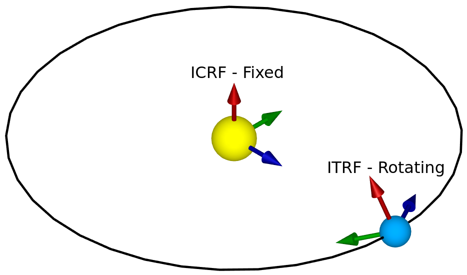
Tracking things in space from the surface of Earth often requires converting between these two frames. However, a frame centred on the Sun like ICRF isn’t necessary for tracking the Moon – for that we need an Earth Centred Inertial (ECI) frame (which is centred on Earth but doesn’t rotate with it) in addition to ITRF.

First, to convert between ITRF and ECI we need to define our axes. We’ll be using a cartesian coordinate system called Earth Centred, Earth Fixed (ECEF) for ITRF, and something very similar but non-rotating for ECI. In ECEF, (0, 0, 0) is at the centre of the Earth, the Z axis points towards the north pole, the X axis points towards the point where the prime meridian touches the equator (GPS 0, 0), and the Y axis points 90 degrees east of that.

There are several steps to the conversion between ITRF and ECI, but because ITRF is rotating and ECI isn’t, we need to know the precise time whenever we convert between them. There’s a reference time called J2000, and we know the exact angles between the two frames at that exact time. From there we can use the speed of the Earth’s rotation (and other things) to figure out what the angles are at any particular time.

Unfortunately, the definition of our reference time J2000 is already quite confusing: it was originally defined as midday (not midnight, because astronomers observe at night) on the 1st of January in the year 2000. However, this was defined in Terrestrial Time, which (a) is an ideal that can’t be measured by real clocks, and (b) differs from UTC by around 32.184 seconds, so the actual value of J2000 is 11:58:55.816 UTC on the 1st of January, 2000. It’s worth noting that at the time of writing we have had 5 leap seconds since J2000 – not accounting for those could throw the calculations off, as leap seconds are designed to keep UTC in sync with the Earth’s rotation.

Next, let’s clarify which ECI we mean, because so far we’ve only said it’s an inertial frame centred at the centre of the Earth, not where the axes are. We have two planes we could use: the equatorial plane (which forms Earth’s equator) in the orientation that it was in at the moment of J2000, and the ecliptic plane (which the Earth orbits the Sun in), they differ by around 23.4° because of Earth’s axial tilt. Since the orbits of all of the planets and the Moon are usually defined in terms of the ecliptic plane, we’ll use that. We’ve decided that the Z axis points up from the ecliptic plane, and we can say that the Y axis is 90 degrees east of the X axis, but we still need to define the X axis. We can do this based on where the prime meridian was pointing at J2000, but the normal definition is actually based on where the mean vernal equinox was at J2000.

The vernal equinox happens in March every year, at the moment when the line that forms the intersection between the ecliptic and equatorial planes points directly towards the Sun. You’ll notice that this is in March, while J2000 is in January – the X axis is based on where the equinox line (i.e. that intersection of the two planes) is in January. The equatorial plane slightly changes over time because of slight variations in the Earth’s axis, which means the direction of the equinox line is constantly, but slowly, changing. Notice that since our X axis is along this line at J2000, we can perform a simple rotation around the X axis to compensate for the Earth’s axial tilt and convert between this ecliptic ECI frame (where the Z axis points upwards from the ecliptic plane) and an equatorial ECI frame (where the Z axis points towards the north pole).

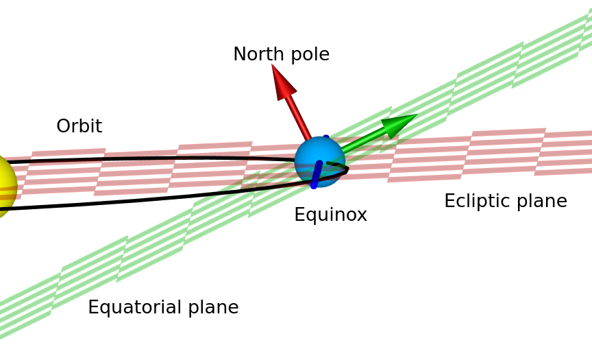
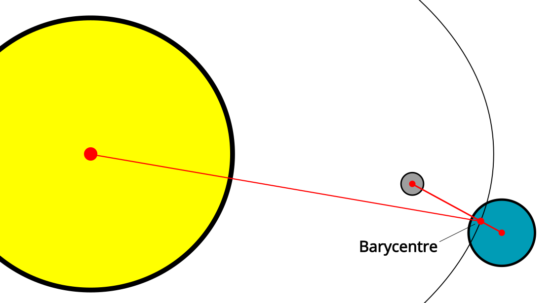
The equinox line (blue, defining the X axis) at a random point in the Earth’s orbit around the Sun. The date in this diagram doesn’t coincide with the date of the equinox (when days and nights have an equal length), because the line is not currently pointing at the Sun.

Now that we have some reference frames defined, we can start to use them.

Finding the Moon’s Orbital Parameters

Code link: moon_orbit.cc

You might have heard that the Moon is very slowly drifting away from Earth at the rate of a few centimetres per year. This is only one of the ways that the parameters of its orbit are changing: it is constantly affected by its orbit around the Earth (which moves it closer to and further away from the Sun), the Earth’s orbit around the Sun, and potentially other things too.

The Keplerian Orbital Parameters are six numbers that can exactly define an elliptical orbit of one body around another. They are:

• Semi-major axis: the radius of the orbit at its widest point
• Eccentricity: the scale of how elliptical the orbital ellipse is (0 meaning circular, 1 and over meaning that it’s not orbiting any more)
• Inclination: the angle of the orbital plane with respect to some reference frame (in our case, the ecliptic ECI frame)
• Longitude of Ascending Node: the angle around the thing we’re orbiting (from some reference direction) where we measure the inclination from. Specifically, this is the angle where the Moon moves from below the Ecliptic plane to above it.
• Argument of Periapsis: the angle around the orbit from the Longitude of Ascending Node where the two bodies are closest to each other.
• Mean Anomaly: the current angle of the smaller body around the larger one, if you assume that the orbit is circular and the smaller body is moving at a constant speed around the larger one. (This is useful because it generally increases uniformly over time, and it can be used to calculate other parameters called the Eccentric Anomaly and True Anomaly, which are actual angles around the orbit).

For a much more in-depth and interactive explanation of how these 6 parameters work together see this page: https://ciechanow.ski/gps/#orbits – it’s geared towards explaining in detail how GPS works, but as part of that it goes into detail on all of the orbital parameters.

For the Moon, all six of these parameters vary over time. The best data source I could find for this was the JPL Horizons tool, which allows you to choose any body in the solar system and get a table that includes more than just these parameters for any range of dates/times.

To begin with, I downloaded all of the Moon’s orbital parameters at a daily resolution for 16384 days starting at midnight on the 1st of January 2000 (unfortunately, due to the way the data is exported, all of the dates were offset by -0.5 days from J2000, but this is correctable).

To analyse this large dataset, I wrote some code in Python to display graphs and do some numeric analysis. The first part of this was to perform a Fast Fourier Transform (FFT) to see which frequencies each component oscillates at. I manually gathered the top 8 frequency components from the graph of each FFT, since the aim is to find a good approximation rather than storing all of this data. For the semi-major axis, eccentricity, and inclination, just an FFT was enough. But the longitude of ascending node, argument of periapsis, and mean anomaly all have linear components too (i.e. the angle has a cumulative increase/decrease as well as oscillations), and their angles always wrap around when they get to 360°. To correct for this, I used a function in scipy called unwrap() with the period set to 360, which turns a time series like the one on the left into the one on the right.

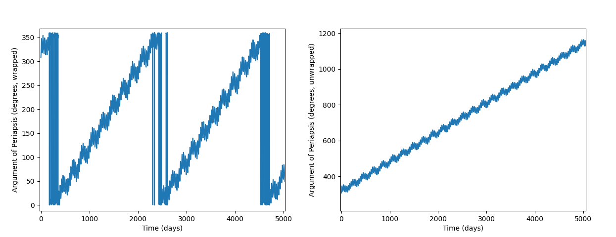
And because this still has a linear component, I first approximated the linear gradient and subtracted it out before performing the FFT. From there, all six graphs look similar, although each have different oscillations.

Finding the initial frequencies was as simple as looking them up in the FFT graphs:

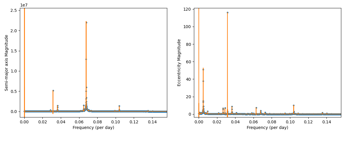
Next, I used a function similar to the following to define the curve-fitting process:

$$a_t = \sum_{i=1}^{8} (S_i sin(2 \pi F_i t) + C_i cos(2 \pi F_i t))$$

Where $a_t$ is the semi-major axis at time $t$, $F_i$ represents one of the eight frequency components (I chose 8 as an arbitrary trade-off between accuracy and complexity), and $S_i$ and $C_i$ are sine and cosine amplitudes. The parameters to optimise are $F_i$, $S_i$, and $C_i$. Using sine and cosine amplitudes is equivalent to using a magnitude and a phase, but it gives each of the parameters a differentiable effect on the output, which makes it easier to optimise than a phase angle. It’s possible to turn the sine and cosine amplitudes into magnitude and phase using the following transformation (example in desmos):

$$magnitude = sqrt(S^2 + C^2)$$

$$phase = atan2(C, S)$$

Functions like the one for $a_t$ above, with some additions for dealing with constant and linear components, were used as the input to scipy.optimize.curve_fit() to find the final parameters, which consist of:

• Eight frequency components, for each of the six parameters.
• Eight sine and eight cosine amplitudes, for each of the six parameters, which we use to calculate the magnitudes and phases using the formulae above.
• A constant offset for each of the six parameters.
• A linear time-multiplier for the Longitude of Ascending Node, Argument of Periapsis, and Mean Anomaly parameters.

We have now optimised these six functions on 16384 days (or just over 44 years) of data from 2000 to 2044. Testing it on the next 16384 days of data from JPL Horizons showed that it fits reasonably well. From there, we can calculate with reasonable accuracy the orbital parameters of the Moon at any point in at least the next ~70 years, but likely much longer.

Keplerian Orbits

Code link: keplerian_orbit.cc

So, how do we use these six orbital elements to calculate the position of the Moon? This is heavily based on NASA’s documentation here about finding the approximate positions of planets, but it applies to any Keplerian orbit including the Moon’s (if you have accurate orbital elements).

First, we need to find the x and y positions in the Moon’s orbital plane, and for that we need to find the Eccentric Anomaly ($E$) from the Mean Anomaly ($M$) and the Eccentricity ($e$):

$$M = E\ -\ e \cdot sin(E)$$

It’s not possible to solve this numerically for $E$, but we can approximate it using Newton’s method. We’re trying to find $M\ -\ E + e \cdot sin(E) = 0$, so let’s set:

$$F(E) = M\ -\ E + e \cdot sin(E)$$

$$E_0 = M\ -\ e \cdot sin(M)$$

(I suppose setting $E_0 = M$ might work too.) Then we can iterate this:

$$F'(E) = -1 + e \cdot cos(E)$$

$$E_{n+1} = E_n\ -\ F(E_n) / F'(E_n)$$

Repeating this until the delta ($F(E_n) / F'(E_n)$) is small enough gives us a good approximation of $E$. Then, we can use the eccentric anomaly $E$, the eccentricity $e$, and the semi-major axis $a$ to get $x$ and $y$, and our $z$ starts at the origin:

$$x = a (cos(E)\ -\ e)$$

$$y = a \sqrt{1\ -\ e^2} \cdot sin(E)$$

$$P_{initial} = (x, y, 0)$$

From there, we just need to rotate these coordinates into position. In my implementation, I used quaternions (extremely useful tutorial here) for this because they are a nicer way of representing arbitrary rotations and they’re easier to read than complex matrix multiplications. However, for simplicity below I’ve assumed an equivalent rotation matrix for each step:

$$P_{periapsis} = R_Z(argument\ of\ periapsis) \times P_{initial}$$

$$P_{inclined} = R_X(inclination) \times P_{periapsis}$$

$$P_{final} = R_Z(longitude\ of\ ascending\ node) \times P_{inclined}$$

This gives us $P_{final}$ as the cartesian position in our reference frame, in this case the ecliptic plane centred on the Earth.

Earth’s Rotation

Code links: earth_rotation.cc, and some of cartesian_location.cc

We can calculate the Moon’s position in ECI, but we need it in ECEF. The next step is to convert between them. There are several steps here:

1. Convert from Ecliptic ECI to J2000-Equatorial ECI (based on the J2000 north pole and equator), by applying the axial tilt.
2. Convert from J2000-Equatorial ECI to the ECI frame based on the current north pole and equator, this is known as CEP or “Celestial Ephemeris Pole”. This involves applying axial precession and nutation.
3. Convert from this CEP frame to ECEF, by applying the rotation of the Earth.

The ESA provides a full description of the steps on their Navipedia site, but it provides a lot of technical detail without much context, so I’ll just summarise here.

Step 1 is very simple, since we defined our ecliptic and equatorial planes with the X axis pointing along the line where they intersect, we can just rotate the coordinates by 23.4° on the X axis.

Step 2 is more complicated. The north pole (and therefore the equator) actually move around over time, in cycles on various different time scales. The largest movement is from axial precession, which means that over 26,000 years the Earth’s axis makes one full rotation. This actually means that in 13,000 years, the northern hemisphere will have summer in January and winter in July. It also means that the vernal equinox line by which we define the ECI X axis moves over time, doing a full circuit in 26,000 years.

The other part of step 2, Nutation, is higher-frequency than precession, and it occurs because the forces that lead to precession are not constant, but vary over the course of the Earth’s orbit due to gravity from the Sun, Moon, and planets. Applying it correctly involves using some long lookup-tables.

Step 3 is mostly about the rotation of the Earth on its (now well-defined) axis. There is also a component called Polar Motion, which is a slight drifting of the axis with respect to the Earth’s crust, but it has a tiny magnitude and requires frequent updates to calculate in an up-to-date way, so I’m ignoring it here.

Sidereal time diagram. Xaonon, CC BY-SA 4.0, via Wikimedia Commons.

The Earth rotates on its axis once every 23 hours, 56 minutes, and ~4 seconds. The difference between this and the 24 hours you might expect is because we need to measure the sidereal rotation (compared to ECI) rather than the rotation compared to the direction of the Sun from Earth, which is always changing. The extra 3 minutes and ~56 seconds add up over the course of a year to one extra sidereal rotation.

The details of this rotation on the ESA website are quite confusing. They define $\theta_G$ as the Greenwich Mean Sidereal Time (GMST), in terms of a fixed rotation over time compared to a reference $\theta_{G_0}$. The changing component is based on the current time in UT1 (which is very close to UTC), but they didn’t provide a reference epoch, so I initially assumed it was J2000, but in fact the reference is defined at midnight at the start of the current day. (In retrospect, they also say that $\theta_{G_0}$ is the GMST at $0^h$ UT1, but it wasn’t clear to me where they were counting hours from – what finally made me notice the error was that both $\theta_{G_0}$ and $\theta_G$ account for the sidereal rotation, and they’re added together in the end).

From $\theta_G$ (GMST), we need to correct for nutation again to get $\Theta_G$ (GAST, or Greenwich Apparent Sidereal Time), and then rotate the Earth by that angle. All of the rotation matrices on the ESA website are inverted (they rotate in the wrong direction), and all of the angles passed in to them are negated to compensate. Converting this all to use standardised quaternions for rotation made things much easier to understand.

Finding our own location

Code link: location.cc

To be able to point at some ECEF coordinates, we first need to know where we are. GPS coordinates are polar coordinates, which give a latitude (the angle away from the equator), a longitude (the angle away from the prime meridian), and an elevation (the height above the Earth’s reference ellipsoid).

The ellipsoid can be defined in terms of a polar radius (from the north or south pole to the centre) and an equatorial radius (from the equator to the centre). Obviously the Earth’s height varies much more than a perfectly smooth ellipse, and even sea level doesn’t quite match the ellipsoid. GPS receivers usually give you both an elevation above mean sea level and an elevation above the reference ellipsoid.

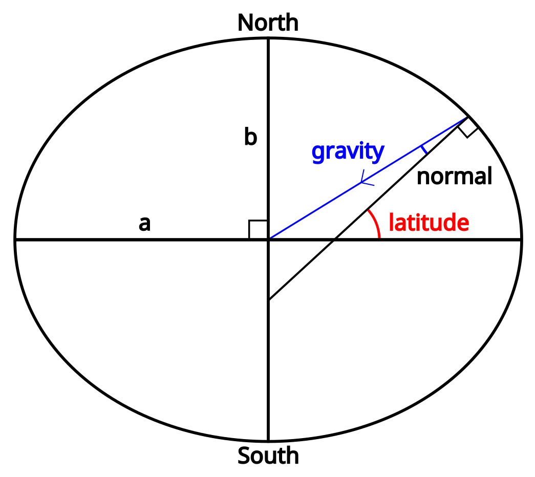
To begin with, it’s worth noting that because we’re not standing on a sphere, a line pointing at a normal to the surface (one of the definitions of “straight down”) doesn’t necessarily point to the centre of the Earth. It’s close, and it does intersect the line going from the north pole to the south pole, but unless we’re actually standing on the equator or the north pole it won’t pass through the exact centre.

The first number we need to calculate is the distance along the normal from our location to the line between the north and south poles. If we call the radius at the equator $a$ and the radius at the poles $b$, this can be calculated as:

$$N(lat) = \frac{a^2}{\sqrt{(a \cdot cos(lat))^2 + (b \cdot sin(lat))^2}}$$

From there, it’s relatively easy to find the $x$ and $y$ coordinates in ECEF:

$$x = (N(lat) + elevation) \cdot cos(lat) \cdot cos(long)$$

$$y = (N(lat) + elevation) \cdot cos(lat) \cdot sin(long)$$

Finding $z$ is slightly more complicated, but doesn’t depend on the longitude:

$$z = \left(\frac{b^2}{a^2} \cdot N(lat) + elevation\right) \cdot sin(lat)$$

Pointing

Code link: cartesian_location.cc (specifically, see directionTowards())

We have the coordinates of ourselves and the Moon, now we just need to point from one of them to the other. We can already calculate a vector, but it’s not very useful without some reference to compare it to. We need to know where that vector is pointing in a local coordinate system.

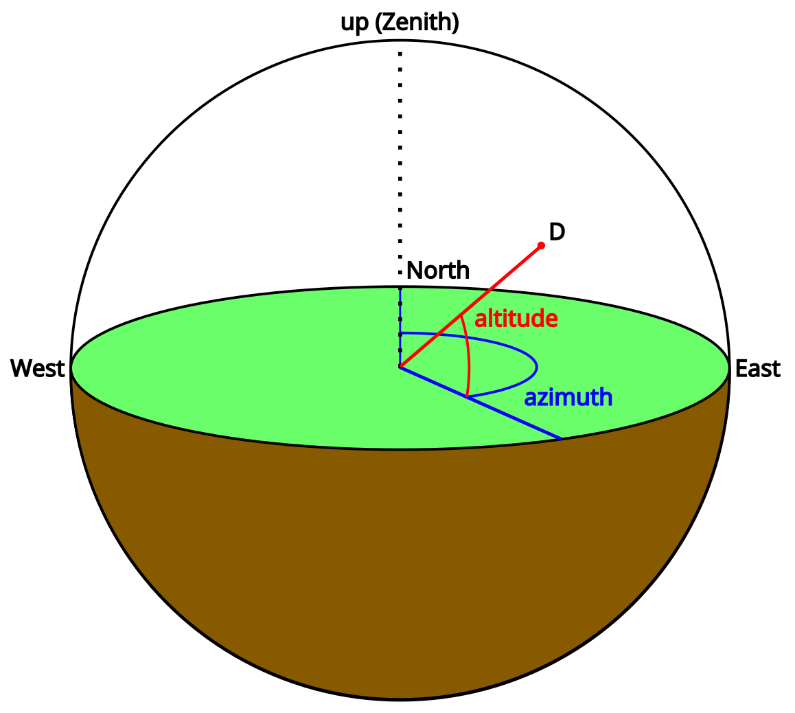
The two angles we need to point at something are often called the azimuth and the altitude. Note that the altitude here is an angle, and not the height above the ellipsoid that I’ve been calling elevation – it seems like in astronomy the term “altitude” is overloaded, and these two terms are often used interchangeably, so I’ve arbitrarily picked “elevation” for height and “altitude” for this angle.

If you’re standing on the surface of the Earth and pointing, your finger’s azimuth is the angle between north and the direction you are pointing (0° = north, 90° = east, etc.). Your finger’s altitude is the angle upwards from the horizon to it. Using these two angles, we can point towards any object in 3D space.

We need a reference direction: the normal to the surface of the Earth ellipsoid at our current location. This is fairly easy to define based on our latitude and longitude:

$$\vec{up} = \begin{bmatrix} x \cr y \cr z \end{bmatrix} = \begin{bmatrix} cos(lat) \cdot cos(long) \cr cos(lat) \cdot sin(long) \cr sin(lat) \end{bmatrix}$$

Getting the altitude from here is simple, given a direction to point $\vec{D}$:

$$altitude = 90\ -\ arccos(\vec{up} \cdot \vec{D})$$

Finding the azimuth is trickier – the easiest way I’ve found is to first rotate both $\vec{D}$ and $\vec{up}$ to the point where the prime meridian crosses the equator:

$$toPrimeMeridian = atan2(\vec{up}.y, \vec{up}.x)$$

The result from atan2() is the anticlockwise angle from the prime meridian, when viewed from the north pole. Our rotations are clockwise around the axis we choose, and we’re looking from the north pole to the south pole, so to remove this rotation we need to rotate clockwise around the negative Z axis:

$$\vec{up}_{prime\ meridian} = R_{-Z}(toPrimeMeridian) \times \vec{up}$$

Next, let’s put this at the equator. This time we’re looking along the positive Y axis:

$$toEquator = atan2(\vec{up}_{prime\ meridian}.z, \vec{up}_{prime\ meridian}.x)$$

$$\vec{up}_{0,0} = R_Y(toEquator) \times \vec{up}_{prime\ meridian}$$

But we aren’t really interested in $\vec{up}_{0,0}$, we already know which way it’s pointing. What we need are those same rotations applied to $\vec{D}$:

$$\vec{D}_{0,0} = R_Y(toEquator) \times R_{-Z}(toPrimeMeridian) \times \vec{D}$$

And finally we can find our azimuth (converting from anticlockwise from east, to clockwise from north):

$$azimuth = atan2(1, 0)\ -\ atan2(\vec{D}_{0,0}.z, \vec{D}_{0,0}.y)$$

Using the azimuth and altitude together, we can figure out which direction to point in, and all we need as references are an up/down vector, and the direction of north. Putting all of this together, we can point at the Moon!

See https://github.com/abryant/CosmicSignpost for the code. There may be more blog posts coming about the motor control code, electronics, and hardware.

Thanks go to my partner Dalia, who pointed me towards scipy and specifically the unwrap function, and helped with analysing the FFTs of the Moon’s orbital elements.

Thanks also go to my Dad, who showed me how to use sine and cosine amplitudes as a more optimisation-friendly formula for the orbital elements than magnitude and phase.

A few months ago, I posted about my LED Cube, which was a 4x4x4 grid of 64 LEDs. Since then, I’ve built a version that’s 8 times as large and twice as dense in each dimension, an 8x8x8 cube:

It has 512 LEDs, four separate signal cables coming from a single microcontroller, and 1824 solder joints. The spacing between LEDs is 2cm (compared to the 4x4x4’s 4cm) meaning that the whole thing is around 16cm to a side. From when I got all of the LEDs to when I finished it, it took around 3 months to make, however the actual time spent working on it was probably in the range of around 100 to 200 hours.

It runs on the same server software stack as the 4x4x4, but with a different microcontroller to download the cube states and display them (which requires some different timing logic, and different signal sending code to write to all four signal lines at once). My git repository is here: https://github.com/abryant/LED-Cube.

Most of this post is some fairly detailed instructions about how to build it / how I built it, with some extra information about how it’s controlled at the end.

Building the Cube

The cube is built of 8 layers, each of which is 8 strips, each of which contains 8 LEDs.

A strip

Each LED has four wires: Data out, GND, +5V, Data in, in that order. The first thing to do is connect all of the LEDs to a power supply, which also serves as the structure holding them up. I used a block of polystyrene (which came with the soldering iron) to hold the LEDs in place, with one of the pins of each LED sticking straight down into it:

Here, the longer ground wires are along the bottom, the shorter +5V wires are along the top, and the data pins go up/down in alternating directions (more on that later). The marks are where the last two LEDs needed to go. Next, we need to solder the rails on the +5V and GND lines, which involves straightening the wire. For this, I am using 22 gauge galvanized steel wire:

1. Cut the wire to length from the reel. This requires two 16cm pieces of wire for a single strip, or 16 pieces for all of the strips in a layer.
2. Straighten the wire by putting it between two pieces of card (I used a greetings card I had lying around), and pressing down on the card while pulling the wire through with some pliers.
3. Finish straightening the whole set. The 90 degree bend at the end of the wire is partly for pulling it through the card with the pliers, and partly to secure it to the polystyrene while soldering.

Next, the wire can be placed on top of the LEDs pins for +5V and GND. They need to be very close to the LEDs so that the layers can be 2cm apart later on:

Note that the data pins go in alternating directions: the first LED has its Data In pin going down into the polystyrene, and the second has its Data Out pin going down.You can see this in the following photos. Note that the side of the LED with the flat edge is the side with the Data Out pin, so the order is: “Flat edge, Data Out, GND, +5V, Data In, (Round edge)”

The reason that the LEDs alternate in direction is so that the data pins can all tie together into one continuous line going in one direction. This will be more clear when we solder 8 strips into a layer.

At this point, the strip is finished, and it needs testing because occasionally one of the colours on an LED won’t work. I did this by connecting the strip to a breadboard with a 5V power supply. Each LED draws around 60 milliamps at full brightness, meaning that a strip can draw 480mA, so a good USB power supply should be enough. To test the LEDs, I moved the data cable between the LEDs’ Data In pins while running a test program. The test program is a very simple one that cycles between red, green, and blue every half-second (it ran on a Raspberry Pi, with a USB cable connected to an Arduino Nano that sent the data signal).

Here’s a photo of an old version being tested (this was when I was originally using 4cm gaps between LEDs):

Note that the LEDs hold their colour when the data cable is not connected, so I’ve set them to an RGB pattern by disconnecting the data cable from each at the right time.

A layer

Once we have 8 strips, we can solder them together to make a layer. Here’s a diagram of how they fit together:

This requires careful alignment to make sure each strip is exactly 2cm from its neighbours all along its length.

1. Use the uncut ends of the GND or +5V pins to stick each strip into the polystyrene. They should all be the same way around, so let’s assume all of the GND pins are facing down. It may take a lot of adjustments and careful measurements to ensure that the 2cm gap is maintained between all of the strips.
2. Take four more straightened 16cm pieces of wire (with 90 degree kinks at the ends), and lay two of them across the top of the strips, connecting all of the +5V lines. There should be one half-way between the 1st and 2nd LEDs, and another half-way between the 7th and 8th LEDs. When positioning these pieces of wire, make sure that the end with the 90 degree kink is always on the right hand side, and as far away from the LEDs as possible while allowing all 8 joints to be soldered. This will give us some extra wire to work with when we are soldering the layers together later on.
3. Solder the two pieces of wire down to the strips, making sure to measure the 2cm intervals after every joint. Once this is done, all 8 strips should be attached on the +5V side.
4. Pull the layer out of the polystyrene and flip it over to do the other two pieces of wire, which will connect the GND lines.
   At this point, the layer will have a common +5V plane and a common GND plane, but the data line will not be connected.
5. To connect the data line, bend the pins into the right positions as shown in the diagram above, and then use some wire cutters to trim each pair (that need to be connected) to length. It’s easiest to trim both of the pair at the same time. After all of them have been trimmed, they can all be soldered together, which completes the first layer.

On alternating layers, the strips need to be made with the data pins going in the opposite direction. This allows the data line to be reversed for the 2nd, 4th, 6th, and 8th layers, which ensures that the signal can go through them after it gets to the end of the 1st, 3rd, 5th, and 7th layers.

Once a layer is finished, it can be tested. Each layer contains 64 LEDs and each LED draws a maximum of 60mA, so the power supply for the test needs to supply 3.84A at 5V. One good test program for a layer is to draw a moving line of colour through the LEDs.

A cube

Once you have 8 layers, they can be connected together into a cube.

But first, they need trimming so that the +5V and GND pins do not interfere with the other layers:

To put the layers together:

1. Decide which direction you want the layers to connect together in. (I forgot to do this, accidentally connected them from right to left, and had to flip the direction of the layers in software afterwards, because it was the opposite of my 4x4x4 cube.)
2. Line up the layers in some polystyrene in approximate positions (they don’t need to be accurate yet). The layers should alternate in data signal direction, so that odd layers have their signal going upwards and even ones go downwards.
3. Put four new pieces of straightened 16cm wire along the GND and +5V lines that are sticking out of the sides. These four wires should be as close to the LEDs as possible without touching any other wires (make sure they’re not too close to the data lines).
4. The four lines can then be soldered to the first layer. It may be easier to remove the layers from the polystyrene before soldering the second layer, because the alignment is very difficult to get right at this stage, and it can be easier to solder each joint separately.
5. Solder the rest of the layers onto these four lines, being very careful that they are connected at 2cm intervals, and that the layers are aligned horizontally and vertically.
6. Solder the Data Out pin at the top of every odd layer to the Data In pin at the top of the next even layer. This will produce four sets of two layers that can be controlled independently. The inputs to each of these four pairs of layers will come from four pins on the microcontroller.

Here’s a cube with only three layers soldered on:

It’s important that two adjacent layers don’t touch, because one layer’s +5V plane is very close to the next layer’s GND plane.

Here’s the full cube after soldering:

Powering the Cube

At this stage, you should have a single cube of 512 RGB LEDs with a common ground and +5V line. However, this cube can draw up to (512 x 60mA =) 30.72 Amps! It will not turn on with a power supply that can’t supply a large current. Additionally, the wire connecting the LEDs together is fairly thin and probably won’t support a full 30.72A of current without heating up a lot. So to turn this on, we need some way to distribute a lot of power around the cube.

The way I decided to do this was to buy two thick pieces of copper wire (one with red insulation, one with black) with enough conductance to support the whole cube. I then stripped the insulation from the middle(-ish) of each piece of wire, and soldered it along the bottom +5V and GND lines connecting the layers together.

I then collected the two ends of each wire and secured them into the terminals on the power supply (I measured my wires so they each had the right amount of slack to reach it). My power supply is a brick that supplies 40A at 5V and has three terminals for +5V and three for GND, so it can cope with the power and logistical requirements.

Controlling the Cube

The cube isn’t very interesting if all it does is show the blue colour that the LEDs default to. The microcontroller attached to it is what allows it to display more interesting patterns, however the microcontroller I use is also fairly simple: it just connects to my server using a wireless internet connection and displays whatever the server tells it to. This allowed me to make a web interface and control the cube from my phone, but it does require a constant internet connection and can eat up some data (at 20 frames per second, it uses around 30 KB/s).

Client hardware

The client I use for the cube is an ESP-12E module, which has an embedded wireless chip and a 160Mhz processor.

As I mentioned in my previous post, the timing for the APA106 LEDs is fairly precise, and needs a signal pulse every 1710 nanoseconds (of either 350ns for a zero bit, or 1360ns for a one bit). This requires some circuitry that can cope with fast changes without suffering from interference.

Annoyingly, the ESP-12E works at 3.3V rather than 5V, so I had to use a voltage regulator to convert the cube’s 5V power supply down to 3.3V first, and then use some transistors to pull the signal wires it outputs back up to a 5V signal (which actually inverts the signal at the same time, so the code has to send 0 when it means 1 and vice versa).

To make sure power supply is smooth and doesn’t suffer from any interference, I have both a ceramic capacitor and an electrolytic capacitor in parallel across it.

To convert the signal from the four data-out pins from 3.3V to 5V, I’m using four n-channel MOSFETs and four 470Ω pull-up resistors. Here’s the circuit diagram (click to zoom):

Client software

The ESP-12E (which uses the ESP8266 chipset) can be programmed as an Arduino device. While it doesn’t support the instruction timing that I used in the Arduino Nano program, it is fast enough that it can count the clock cycles itself. It also has enough spare cycles to calculate four different output signals at once, which decreases the time required to update the cube by a factor of 4, from ~21ms to ~5.25ms. It takes this long because there are 512 LEDs to update, each of them need 24 bits of colour data, and each bit takes 1710 nanoseconds to send: 512 x 24 x 1710ns = 21,012,480ns ~= 21ms. Since interrupts must be disabled while sending the signal to the cube, pausing for 5.25ms is much more feasible, especially when we want to update at 20-30 frames per second and we’re waiting for data from the wireless network at the same time.

There are some really useful Arduino libraries for WiFi management. The one I’m using will auto-connect to the last network it connected to, but if it fails for some reason or can’t connect to the server it will start up its own network with a captive portal that lets you scan for networks and enter the password to one, after which it will connect to that network and continue from there.

The full client code is here:
https://github.com/abryant/LED-Cube/tree/master/arduino

Server software

The server is a multithreaded Python HTTP server. When a request comes in from the cube, it registers that the cube exists and starts a controller that keeps the connection open indefinitely to send frames to. The web interface sends commands via POST requests, and when one comes in the controller responds by changing what the cube is doing, for example by changing the current visual displaying on the cube. When a non-interactive visual is running, the controller just gets the next frame 20 times per second (or at whatever speed the controller has been set to). Interactive visuals are handled differently, and can respond to other POST requests from the web interface.

The visuals themselves are python generator functions (similar to an infinite iterator, but much easier to write) that yield Cube objects or lists of colours. A Cube object is a 3D array of colours with some utility functions that let the visuals do interesting things. The visuals themselves can be quite short pieces of code, for example “Layers” is less than 30 lines, and more complex ones like “Faces” and “Snakes” are less than 100 lines of code. “Starfield” has about 5 lines of actual non-boilerplate code.

The visuals can also be chained together in sequences, using some generator utilities (which is what’s happening in the video above). Whenever a generator yields a boolean value, the generator utilities treat it as a break point and have the option of moving on to another visual, or doing something else.

The server also sends the current state of the cube to any listening instances of the web interface, which then draws it on screen:

This cube was a lot of fun to make, and I’m still experimenting and improving it with software (e.g. new visuals) and hardware (e.g. ways to cool the LEDs when they’re at full brightness). It taught me about soldering (I hadn’t soldered for about a decade), building circuits, Arduino programming, Python web servers and generators, WebGL, and probably lots of other things.

Thanks to everyone who helped me, and to those who came up with ideas for visuals to display on it. Special thanks to my grandfather James M. Bryant without whose help I wouldn’t have known about APA106 LEDs, the ESP-12E, or the various bits of electronics I needed to put the whole thing together.

I have a few ideas for new visuals, but I’m always interested in more – feel free to send me ideas, or even better, write code for them and send it to me!

I’ve been building a cube recently:

It’s built from 64 programmable LEDs (in a 4x4x4 lattice), that I can control with a serial signal from a 16MHz Arduino. More specifically, these are APA106 LEDs, which have a chip embedded inside them that decodes the signal and outputs the programmed colour levels to the LED. They take a 3-byte RGB signal, which in theory means 16,777,216 possible colours (although your eyes can only see around 10 million).

Each LED has four wires: Data out, GND, +5V, Data in (left to right in the picture above). The 5V supply and ground pins are the main power source, and the 64 LEDs in the cube are connected to the supply in parallel. The Data in and Data out pins, however, run in series through the whole string of LEDs – the first LED’s Data out pin connects to the second LED’s Data in, and so on. Only the first LED in the sequence gets a signal from the Arduino, and once it has received its colour it propagates the rest of the serial signal on to the LED after it. Because all of the LEDs work this way, you can just send a sequence like R1,G1,B1,R2,G2,B2,R3,G3,B3,… to update all of the LEDs at once.

In the video above, all 64 LEDs in the cube are being updated 20 times per second. For parts of it, you can see a rainbow pattern weaving its way through each of the LEDs in turn. The order in which the LEDs turn on/off there is the order in which the data pins of the LEDs are connected to each other.

At maximum brightness, each LED draws about 60mA of power at 5V, meaning that the whole cube draws 3.84A. Most USB ports and phone chargers only supply one or two amps, so here I’m using a separate 5V 10A power supply. The Arduino is still powered over USB, so to connect the data wire safely I had to also connect the two ground wires together, but not the 5V.

The timing on the signal needs to be fairly precise, according to the APA106 datasheet the smallest time between signal changes is 350ns with an error of up to ±150ns. Initially, I tried to do this from a Raspberry Pi’s GPIO pins, but my program would always get interrupted in the middle of sending the signal, so I had to use an Arduino instead. I adapted some signal sending code for a similar type of LED I found online, which disables interrupts and uses assembly code for instruction level timing based on the fact that the processor runs at 16MHz.

In order to write visualisations in a higher level language than Arduino C, I wrote a very simple Arduino program that listens for data on USB and forwards it to the LEDs with the correct timing. The USB signal has a maximum baud rate of 115200, meaning that I can send a maximum of 115200/(64x3x8)=75 updates per second to the whole set of 64 LEDs. In practise, I’m only sending 20 per second.

To send those signals and generate interesting patterns, I’ve written some Python programs that run on a Raspberry Pi, which the Arduino is plugged into. These programs generate one frame after another and send them to the Arduino at 0.05 second intervals.

You can find the code, including Python visualisations and the Arduino LED controller, on my GitHub here: https://github.com/abryant/LED-Cube

Some of the visualisations I’ve written so far are:

• A rainbow filling up the cube in LED order.
• Blocks of colour scrolling past in different directions.
• One face of the cube rotating to become another face and changing colour.
• A 3D game of snake.
• Tetris blocks falling in random places until they reach the top.
• Pulsing the whole cube in different colours.
• Falling green lights (matrix-style).
• A rotating 3D colour wheel.
• 3 different coloured snakes all avoiding each other.

You can see some more photos and videos here:
https://photos.app.goo.gl/b63fNjHddFoOuM0C2

Unfortunately, some of these don’t work very well because the cube is so small. 4x4x4 isn’t enough to display much detail, for example you can’t display text on it. To remedy that, I’ve started building an 8x8x8 cube with 512 LEDs. Hopefully I’ll put up some more detailed blog posts about the construction and soldering as I go.